Using Excel as a Grade book

Grade book basics

Many school systems have begun to provide grade recording software applications to their teachers. If your school system does not provide such software to you, perhaps you could make your own grade book using Excel.

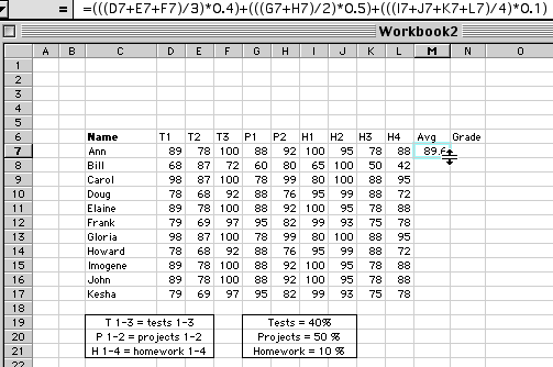
Below you see an image of the beginning of a Grade book Several elements of this image will be discussed one at a time. Your grade book may be more simple than the example below. We purposely used a fairly complicated weighted grading system to illustrate the things that you can do with Excel

Send Email to either of the co-founders of Internet4Classrooms if you need specific help in making, or modifying, a grade book for your own classroom management.

Our email addresses can be found at the bottom of any of our pages.

This is not shown so that you can copy my information into a spreadsheet. It is Only shown as an example.
As you experiment with using an Excel workbook as a Grade book, you should keep it simple.
Start with 4-5 names and at most two types of grades.

Legend

Legend - List each item for which you gave a grade. Be specific, you have plenty of room and later you may wish that you had recorded more information about what assignment the grade was given for.

Grade Policy

Grade Policy - You should clearly spell out how you will use grades to determine a student's final grade. An Excel worksheet provides enough room that this information could be included on each Grade book page.

Function

Equation for determining grades (Function) - The equation above applies my stated grade policy. If you can state your grade policy as an equation, you can write an Excel function to do the calculation. The function above does the following

• Test grades
  • Add the three grades (D7+E7+F7)
  • Divide by the number of grades (average)
  • Multiply by 0.4 (40 %)
• Project grades
  • Add the two grades (G7+H7)
  • Divide by the number of grades (average)
  • Multiply by 0.5 (50 %)
• Homework grades
  • Add the four grades (I7+J7+K7+L7)
  • Divide by the number of grades (average)
  • Multiply by 0.1 (10 %)
• Filling the function into other cells - In the sample worksheet above the function has been entered into cell M7. Click on the bottom right corner of the cell and drag down to the last cell where the function is needed. In the example above that would be cell M17.

Formatting data

Averages can be displayed to whatever precision you wish to use. I used one decimal place, although you may wish to use zero decimal places. Zero decimal places would keep the grades in a format like they are reported to students. An advantage of using zero decimal places would be to avoid confusion regarding rounding grades. To illustrate this consider the following grade:

• A grade of 75.49 would round to 75 with zero decimal places. However, at one decimal place that grade rounds to 75.5 and students would have the expectation that the grade would round to 76. Using zero decimal places will allow Excel to round without confusion to some students.

How to format

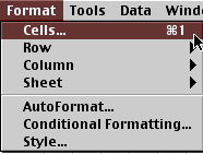
1. Highlight the column to be formatted by clicking on the letter at the top of the column.

2. From the Format menu choose Cells

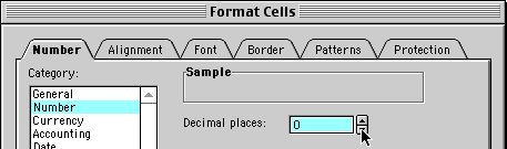
3. From the Format Cells window choose Number and then select the number of decimal places you want to use.

Advanced Grade book topics

Using a Lookup table

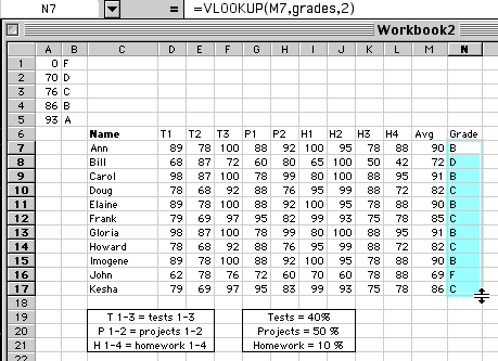
Now we will ask Excel to look at the numerical average in column M and compare it to a list which defines the grading scale, for the purpose of assigning a letter grade to the average. Room was left at the top of the Grade book for this purpose.

The information to the left, defining the grade scale must be entered in ascending order from top to bottom. The number entered to the left of a letter must be the lowest number grade that would equal that letter grade.

1. enter the numbers and letters
2. highlight the entire range from A1 to B5
3. Go to the Insert menu, select Name and choose Define
4. Give a name to this lookup table, I called mine grades

Next we will write an equation which will look at a student's numerical average, look at a list of grades, and assign a letter grade to the student. This is done with a functioned named VLOOKUP. The equation must specify three elements:

1. The location of the numerical grade to be compared (M7 in the example)
2. The name of the lookup table (grades)
3. The location of the letter grade in the lookup table (2) [because the letter grade is in column 2 in the lookup table]

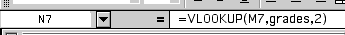
After the equation is entered in N7, click and drag to fill the equation down into the remainder of the Grade book

A List of Online Resources for Excel Grade books

1. Microsoft Template Gallery for Teachers Step by step Tutorials - PDF Files.
2. Part one - Part Two - Must get both to get the entire tutorial
3. Microsoft in Education: Excel 2002 - Microsoft Tutorial - Managing Grades
4. Excel Grade book: Other Helpful Calculations - University of Wisconsin-Eau Claire - Scroll to the Grade book section.
5. How to Use VLOOKUP Excel Formula - Data lookup is one of the most important processes to understand if you want to analyze your data optimally
6. The Last Guide to VLOOKUP in Excel You’ll Ever Need - six easy steps