Using an Excel worksheet - Automatic Features

Using Excel X for Mac

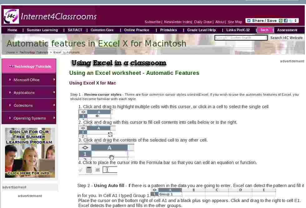
Step 1 - Review cursor styles - There are four common cursor styles used in Excel. If you wish to use the automatic features of Excel, you should become familiar with each style.

1. Click and drag to highlight multiple cells with this cursor, or click in a cell to select the single cell

2. Click and drag with this cursor to fill cell contents into cells below or to the right.

3. Click and drag the contents of the selected cell to any other cell.

4. Click to place the cursor into the Formula bar so that you can edit an equation or function.

Step 2 - Using Auto fill - If there is a pattern in the data you are going to enter, Excel can detect the pattern and fill it in for you. In Cell A1 I typed Group 1.

Place the cursor on the bottom right of cell A1 and a black plus sign appears. Click and drag to the right to cell E1. Excel detects the pattern and fills in the other groups.

The image below illustrates some other patterns, and a problem with this procedure:

In row 3 the procedure did not work because there are too many possibilities. In cell B5 I typed the 2, highlighted both cells A5 and B5, clicked and dragged to the right. Now that Excel knew the pattern it could fill in the cells.

Note : This procedure works in two directions only. You may fill to the right or down . Auto Fill will not fill to the left or up .

Step 3. Using Auto Sum - Excel allows you to quickly find the total of a column or row of numbers.

Step 1 - Select the cell below your column of numbers (or to the right of your row of numbers).		Step 2 - Select the Auto Sum button from your Standard toolbar

	Step 3 - When you verify that the range of numbers is proper, depress return/enter and the sum is displayed.

 

Step 4. Problems Using Auto Sum - Excel will automatically do what it is set to do. In this case, the program finds all adjacent numbers in a column, or row, and includes them in the range.

Step 1 - If there is a gap in the data, Excel will highlight only numbers not separated by an empty cell.		Step 2 - Place your cursor in the highlighted equation and click to edit. In the example above I would change A4:A5 to A2:A5

	You may also click into the equation in the formula bar above the worksheet, and make changes there.

 

Step 5. Using Merge and Center - For giving a clean design look to your worksheet, consider using Excel's Merge and Center feature. This is a two step process:

1. Highlight a range of cells
2. Select the Merge and Center button
3. If you have data in only one cell, that data will be in the center of one long cell.
   

If you attempt to Merge and Center with data in more than one cell, you will wipe out data in all but the upper-leftmost cell. Don't worry, Excel will warn you!

Next Module: Worksheet Basics - Using functions