Making a Review Quiz with Excel

Using Conditional Formatting and Drop-Down Lists

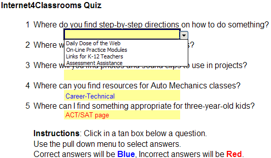
Make a review quiz in Excel and format the cells so that right answer selections are a different color from wrong answer selections. The image below is a sample of what the quiz would look like. Question 1 shows what the drop down list would look like and questions 4 and 5 show what right and wrong answer choices would look like.

When you have composed your quiz questions and answer selections, open an Excel workbook and scroll past where the screen would be displayed when the Excel workbook opens. In my sample below, I scrolled over to column heading AA which is just past Z . The questions are not necessary, but I found that it helped me to have them on the sheet. Type your questions and answers, or type the questions and answers you see below.

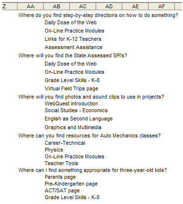
After you have typed your questions and multiple choice answers, scroll back to the beginning of the sheet and put the title of your quiz in cell A1 .

My question numbers started in cell A3 , and I skipped a row between each of the numbers. Next, move over to column B to start typing your questions. Excel will not word wrap. You can add carriage returns, but that will not be necessary. Just ignore the grid lines, we will remove those later. If you typed your questions in the AA area of the worksheet, scroll over to that area, click in the cell with a question and copy the question. A quick way to copy is to hold down the Ctrl key while you tap one time on the C key. ( Ctrl + C ) Next scroll back to cell B3 to paste the first question. Click into cell B3 and paste. A quick way to paste is to hold down the Ctrl key while you tap one time on the V key. ( Ctrl + V ) Continue this process until you have entered all questions. Leave a row between each question.

Put your cursor on the line between column heading C and column heading D . When your cursor turns to a double-headed arrow, click and drag to the right to make column C wide enough for your widest multiple choice answer. Next, click into cell C4 under the first question. Use the fill color bucket ( )to fill the cell with Light Yellow . That is the tan-looking color you see in the image at the top of this page. Repeat that process until all questions of your quiz have a light yellow block immediately below the question.

Making a Drop-Down List

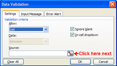
Click into cell C4 , the light yellow block just beneath question 1. From the Data menu select Validation . In the Validation criteria section, click on the down arrow at the right of the box under the word Allow and drag down to the selection List. Clicking on the square with a red arrow in it at the right of the Source box will collapse the Data Validatio n window so you can select the data which will be included in your first drop down list.

After clicking on the red arrow, scroll to the place on the worksheet where you typed the answers. Click and drag to highlight the answers. Remember the answers are only in the cell where you started typing, even though they look like they spread into several columns. In my example I was highlighting only four cells in column AB . If you select some of the empty cells Excel will warn you that the list source must be a reference to a single row or column.

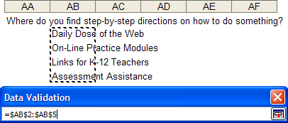
After you highlight the data, click on the red arrow in the Data Validation box to open the box wide and then click on the OK button. Scroll back to the light yellow cell under the first question. At the right end of the cell you will see a down-pointing arrow on the drop-down box. This drop-down arrow is only visible when your cursor is in that cell. Continue this process until all of the light yellow boxes under your questions have had drop-down boxes associated with them.

Using Conditional Formatting to Indicate Right and Wrong Answers

Choose the correct answer to question 1. The answer remains black because that is the default format for text entered in Excel. Conditional formatting allows you to specify a response to content in a cell. You will be asked to list the correct content which must be in the light yellow cell in order to make the text turn blue. The safest way to do that is to copy the answer. Cell C4 does not actually have content in it, it displays a drop down list. However, you can copy the text from the formula bar above. Click in the formula bar, and then click and drag to highlight the right answer. Copy the answer. Remember, a quick way to copy is to hold down the Ctrl key while you tap one time on the C key. ( Ctrl + C )

With the answer copied to the clipboard, go to the Format menu and select Conditional Formatting . In the line where you see Cell Value Is , use the down arrow to change from between to equal to . Then click into the box that appeared to the right of the equal to box and paste the correct answer. Remember, a quick way to paste is to hold down the Ctrl key while you tap one time on the V key. ( Ctrl + V ) Next click on the button labeled Format and in the Color box select a color for the correct answer. Some people use Green for correct and Red for incorrect, reasoning that green implies Go and red implies Stop . To me, the green choices are either too light or too dark for proper contrast. Don't close this window, you are half way through.

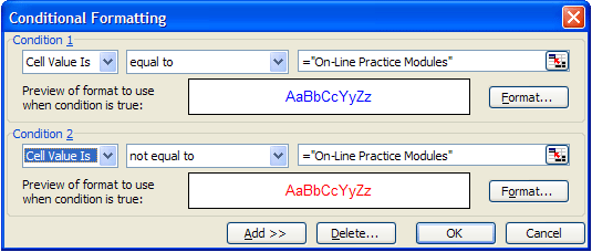
When this box first opens it is only half of this height. After selecting Add >> it opens fully.

Click on the button labeled Add>> . When the Conditional Formatting window fully opens, set condition 2 the same way you set condition 1 . Change the second box to not equal to and change the format color to red . Follow the same procedure for each of the light yellow answer boxes.

One final step will make the quiz look better. Let's remove the gridlines. Go to the Tools menu, slide down to Options and click one time. On the View tab, in the bottom left corner there is a checkmark by the word Gridlines. Click in the box to remove the check mark and then click OK to return to a blank worksheet. The quiz is ready to use.

After a student has taken the quiz and all answers have been selected, click on the light yellow boxes and press the Delete key. This removes the answer, but does not change the formatting. If you wish to select all of them at once, hold down the Ctrl key as you click on the light yellow boxes one at a time. After you have clicked on each one, press the Delete key to remove all answers. Now the quiz is ready for the next student.

Download a copy of the quiz made using these instructions .