Using an Excel worksheet - Calculating Percent and Using Absolute Cell Reference

Step 1 - Review percent - Before showing how to calculate percent with Excel, let's review how to calculate percent.

A number divided by a second number and multiplied by 100 expresses what percent the first number is of the second number. If you do not multiply by 100 you have the decimal equivalent of percent.

Step 2 - Writing a percent equation for only two numbers- Solve the following: 2 is what percent of 8?

Now that you are sure you remember the process for calculating percent, use an Excel worksheet to perform the calculations.

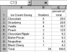
Step 3. Writing a percent equation for a column of numbers accompanied by a sum. - Data from the ice cream survey will be used to illustrate how to calculate percentage.

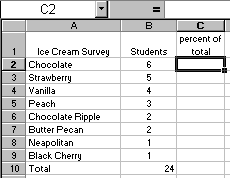
Task: Determine what percent 6 is of 24 by putting the equation into cell C2 of a worksheet similar to the one above.

Step 4. Auto Fill and problems associated with it - You probably remember a discussion of Auto Fill on a previous module . That is a convenient way to place information in several cells at the same time. That might sound like a very good way to fill the equation into cells C3 through C9. For instructive purposes we will do that now to see the problem it causes.

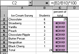
Oops! Something wrong there. The problem was caused by the way the equation was written. The equation B2/B10 says, "take the first cell in this equation and divide it by the cell 8 spaces below." The reason that none of the other equations work is that there is nothing in the cell 8 spaces below any of the cells from B3 to B10. We must find a way of telling Excel to use call B10 to divide by for each of the other 8 equations.

Step 5. Absolute Cell Reference - You tell Excel to use one specific cell, and never move to another relative location in the calculations by using "absolute cell reference." To specify the cell, place a dollar sign before the column letter and before the row number. Thus, $B$10 says always use cell B10. Lets go back to the worksheet and re-write the equation in C2.

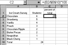
Notice the answer has not changed. If we were writing only this one equation, we wasted time using absolute cell reference. The real benefit of this equation will be seen when you fill down into cells C3 through C10.

Step 6. Fill the equation down into the cells below - If you need to review how to accomplish that go back to a previous module . As soon as you fill this equation with an absolute cell reference down into cells C3 through C10, the percentages are instantly calculated. Only one more task remains.

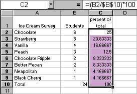
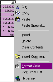
Step 7. Format the cells - Unless you need five decimal places, I suggest formatting cells C2 through C10, the highlighted range above, so that one decimal place is displayed.

Right-click on the highlighted range of cells, and select Format Cells... (Macintosh users, Hold down the Ctrl key while clicking. If you want more information on this see a module about teaching your Mac to right-click .)

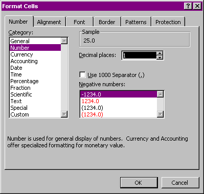
In the category list select Number, and in the Decimal places: box use the down arrow to choose 1.

Click OK, your column of data has a nice uniform appearance.

Return to an index of Excel modules