Using Excel as a Graphic Organizer:

Making a Number Line

Using Excel as a graphic organizer, you can create a variety of documents useful in a classroom. This module will discuss how to create a number line. The number line can be printed and used as a worksheet. However, if viewed in Excel you have some interactive possibilities. If you have classroom projection capability, or an interactive whiteboard, this number line can be really useful.

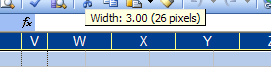
Open an Excel workbook. Click on the column heading A . The entire column will highlight. Scroll over to the right until you can see column heading Z . Hold down your shift key and click on the Z. You should now have 26 columns selected. Click on the line between any two column heading letters and drag to the left until the column width is approximately 3 (26 pixels). When you release the mouse button all 26 columns will be the same narrow width. Scroll back to column A and click anywhere to remove the highlight color. We will use these grid lines as reference points for our number line.

To make the number line you will draw one long thick horizontal line with arrows on both ends. All other lines will be created with the Borders toolbar button. You must have the Drawing toolbar open to draw this line. If the toolbar is not open, go to the View menu, select Toolbars and slide over to Drawing and click one time.

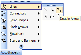
Click on the word AutoShapes in the Drawing toolbar, move your cursor to Lines and click one time on the line with two arrow heads.

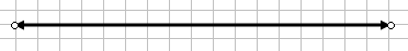
Move your cross hair cursor somewhere near the middle of the sheet, close to the left edge. Place your cross hair cursor on the vertical grid line that is between B and C . Click and drag a straight line (hold down the Shift key to do this) until you get to the vertical grid line between Column headings R and S . While the line is still selected, move your cursor to the Line Style button on the Drawing toolbar and select the thick line labeled 3 pt .

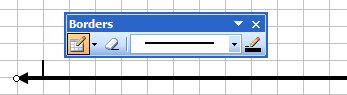
Click in the cell that is immediately above the left arrow head. If you started on the vertical grid line between B and C , the cell will be in column B. We are going to place a vertical line on the right side of that cell by using the Border button on the Formatting toolbar. The button is to the left of the paint bucket. Click on the down pointing triangle to the right of the dashed lines and click on the bottom button named Draw Borders . From the Borders pop-up, click on the down pointing arrow in the Line Style box and slide down to the thicker border just below the double border line. Use the pencil to draw a thick line from top to bottom of the cell directly above the left end of the arrow.

Next, we draw the same line in each of the fifteen cells to the right. However, we will take a shortcut. On the Standard toolbar you will see a paintbrush. This paintbrush is named Format Painter because it can absorb the formatting of something and transfer that formatting to something else. We just formatted a cell to have a right border. With the cursor still in the cell that has a right border, double-click the format painter toolbar button. One at a time click on each of the cells to the right of the starting point until you have reached the arrowhead. Don’t click on the arrowhead. On the row below the number line, put the right border on the cell directly under the first cell, and then every fifth cell until you reach the last cell before the right arrow head.

Students may be confused by a number line without numbers, and Excel will not put the numbers where you want them. To solve that problem we will create numbers in a text box, and they can be moved anywhere you want them. One text box number will be created and formatted the way we want them. Then we will copy, paste, and edit to make the others.

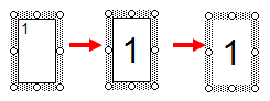
The text box button is on the Drawing toolbar. Click on the button and then click and drag a small box anywhere on the worksheet. Type the number 1. Click and drag to highlight the number and select font size 18 from the Formatting toolbar, and then click on the B (near font size) to make the number bold. There is a gray looking border around the text book, composed of diagonal lines. Click anywhere on the diagonal lines, but not on one of the circles, to turn the border into a series of dots. From the Menu bar at the top, click on the Format menu and select Text Box . On the Alignment tab select Center for both the horizontal and vertical alignment. On the Colors and Lines tab select No Fill for the fill color. You may not see the reason for selecting No Fill, after all, it’s white fill on a white background. If you do not remove the fill color, when moving the number into place the white background may overlap some part of the number line. The image below shows progressive changes made to one of the text boxes used in this project. .

To copy the number, hold down the Ctrl key and press the C key ( Ctrl + C ). After a number has been copied, paste several more of the numbers by holding down the Ctrl key and pressing the V key ( Ctrl + V ) several times. Create the numbers you want for your number line by editing the number in a text box. Click in the text boxes, highlight the number and change it to the numbers you will need; negative values, negative to positive values, multiples of five, whatever you want to use. To move a number first click on the number, then click on the gray box surrounding the number. Now the numbers can be moved with the keyboard arrows or by clicking and dragging.

On the Drawing toolbar click on the word AutoShapes , slide up to Block Arrows and click on the down pointing arrow on the right end of the top row. Use the cross hair cursor to click and drag and draw a long slender arrow. anywhere on the worksheet. Use the Fill Color paint bucket to color the arrow red. This arrow can now be moved by clicking and dragging, or by using the keyboard arrows (if the arrow is selected) to indicate a point on the number line.

You may leave the grid lines in place or remove them. To remove the grid lines, go to the Tools menu, slide down to Options and click one time. On the View tab, in the bottom left corner there is a checkmark by the word Gridlines. Click in the box to remove the check mark and then click OK to return to a blank worksheet.

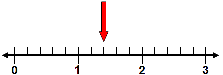
An example of a number line created in Excel is shown below:

Sample workbook

Let us know if you have any other ideas for using this feature of Excel. Bill Byles