Make a Mad-Libs activity using an Excel Workbook

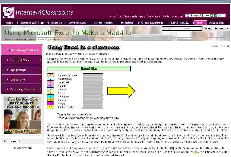
A sample is provided below to help you visualize your final product. For this activity we modified Mary Had a Little Lamb . These instructions are specific to this story, but the procedure can be modified to produce any mad-lib type output.

Open an Excel workbook. Click on the Start button at the left end of the Task bar, go to Programs and then look for Microsoft Office or Excel. The Excel workbook opens with three worksheets; their tabs are at the bottom of a worksheet. Double-click the tab that says sheet 1 and type the words “ type here .” Double-click the tab that says sheet 2 and type the words “ read this .” Right-click on the tab that says sheet 3 and select Delete .

Next we will format text size to 14 in all cells on both sheets. Click on the type here tab, hold down the Ctrl key and click on the read this tab. That selects both sheets. Select all cells on both sheets by holding down the Ctrl key and tapping one time on the A key. Locate the font size box on the Formatting toolbar and use the down pointing arrow to select font size 14 . Right-click on any sheet tab and choose Ungroup Sheets .

Click in cell B2 and drag over to cell I2 to highlight eight cells. Click on the Merge & Center button on the Standard toolbar. The eight cells have become one cell which spans across the space of eight cells. Type Excel-Libs as a title. Use the Fill Color bucket to fill the cell with color. Use the Border button to put a thick border around the cell.

Click in cell B4 and type the number 1 . Press Enter to go to cell B5 and type the number 2 . Click in cell B4 and drag to cell B5 to highlight both cells. There is a black line around both cells. The bottom right corner of the black line is a black box ( ) . When you put your cursor on top of the black box, the cursor turns to a black plus . Click on the black box with the plus cursor and drag down to cell B13 . Let up on your mouse button to see the numbers 1 through 10 filled into the cells. Use the border button to draw borders around the cells, and use the fill color button to fill various colors in the cells. If you click on the down arrow to the right of the Border button you will see one choice that looks like a window with 4 panes . That puts a border around each cell. The down pointing arrow to the right of the fill color button allows you to select different colors.

Click in cell D4 and type the words you see in the illustration above. Press enter to go to cell D5 to continue to type. Follow this procedure until all ten cells have text entered in them.

Click in cell F4 and drag down to cell F13 to select ten blocks. Use the fill color button to fill the cells with gray. Use the border button to draw borders around each cell. Click on the right edge of the F column heading and drag to the right to make the cells wider.

Skip a row below the gray boxes and type the two instructions that you see below the boxes on the illustration on the front of this page.

The final step on this sheet is to draw a large yellow arrow and make it act as a hyperlink to the second worksheet. You must have the Drawing toolbar open to draw this web. If the toolbar is open you will see the word Draw in the bottom left corner of the Excel window. If you do not see the word Draw, go to the View menu, select Toolbars and slide over to Drawing and click one time.

Click on the AutoShapes section of the Drawing toolbar, slide up to the Block Arrows section and slide over to click on the first arrow, the one that points to the right. Move your cursor onto the blank sheet. Notice that the mouse pointer has changed to a cross hair. That is the drawing cursor. Click on the left mouse button, leave the button pressed down, and drag diagonally to the right and down to draw a medium-sized arrow. While the arrow is still selected, use the line thickness button to make a darker line around the arrow. Next, use the fill color button to fill the arrow with yellow.

With the arrow still selected, go to the Insert menu and select Hyperlink. When the Insert Hyperlink window opens, the default choice is Existing File or Web Page . Click on the icon below that, Place in this Document, and select the sheet named Read this .

Another change you might want to make is to remove the grid lines. Go to the Tools menu, slide down to Options and click one time. On the View tab, in the bottom left corner there is a checkmark by the word Gridlines ( ). Click in the box to remove the check mark and then click OK to return to a worksheet with all of the grid lines removed. We needed the gridlines earlier, but now they interfere with the clean look of this sheet.

 

Instructions for making page 2 of the Mad-Libs activity

Next, we will make the page which will display the Mad-Lib poem after the ten words were typed in the gray boxes. Below is a sample of what this page will look like:

Click on the tab labeled “ read this .” The colored borders will be added last. For the sheet above you will type one word per cell. Some cells will be left blank. Those cells will be filled in from the words typed into the gray boxes on the “ type here ” sheet. First, let’s enter the text shown in black above. Enter the words in the following cells: E4 had , F4 a(an) , D6 whose , E6 fleece , F6 was , H6 as , D8 and , E8 everywhere , F8 that , H8 went , D10 the , F10 was , G10 sure , H10 to , I10 go! , D12 It , F12 him/her , G12 to , I12 one , J12 day. , D14 which , E14 was , F14 against , G14 the , H14 rules. , D16 It, E16 made , F16 the , I16 and , D18 to , E18 see , F18 a(an) , H18 at , and I18 school .

Next we will write an equation to fill in the spaces that have red zeroes in them in the image above. There are thirteen places where we will tell excel to fill in the ten words. Some words will be used more than once.

Click into cell D4 . Enter the equal sign to begin an equation. Click on the type here tab, then click into the first gray cell which is F4 and then press the Enter key. This completes the equation and when a name is typed into cell F4 it will show up in cell D4 on the read this page. The next cell on the read this page that needs an equation is G4 . Enter the equal sign to begin the next equation. Click on the type here tab, then click into the second gray cell which is F5 and then press the Enter key. This completes the second equation and when an adjective is typed into cell F5 it will show up in cell G4 on the read this page.

Follow this same procedure for the remaining blank cells that have a red zero in them in the illustration above. Click into the named cell, enter the equal sign, and click on the type here tab and then click into the destination cell in bold type. Beside the following blank cells on the read this page the destination cell (in bold) on the type here page is listed; H4 F6 , G6 F7 , I6 F8 , G8 F4 , E10 F6 , E12 F9 , H12 F10 , G16 F11 , H16 F12 , J16 F13 , and G18 F6 .

Draw a large red arrow and add a hyperlink to the drawing to allow students to return to the type here page.

Save your workbook. When the Save As box appears give the file a name. Before you click on the OK button, change the Save as type box from Microsoft Office Excel Workbook to Template . If a student accidentally changes something you will still have the template to go back to.

If a student follows another student to use the same workbook tell the students to click and drag to select all of the gray cells and then press the Delete key to clear out the previous entries.

Optional instructions to put a colored border around the mad-lib poem

In the column heading row, click on the border between C and D and drag the line to the left, making the C column narrow. Follow the same procedure using the line between columns K and L and drag to the left making column K narrow.

Click in cell C3 and drag down to C19 to select all cells. Use the Fill Color button to fill the cells with a color. Repeat the same procedure for cells K3 through K19 . Next fill the cells in Row 3 from C3 to K3 with the same color. Finally, fill the cells in Row 19 from C19 to K19 with the color. If you want a second narrow band of color around the mad lib poem follow the same procedure after making columns B and L narrow.

Download an Excel file created using these instructions
as an Excel file (.xls) | as an Excel template (.xlt)