Use Excel '07 to Make an Interactive Practice Sheet
using Conditional Formatting

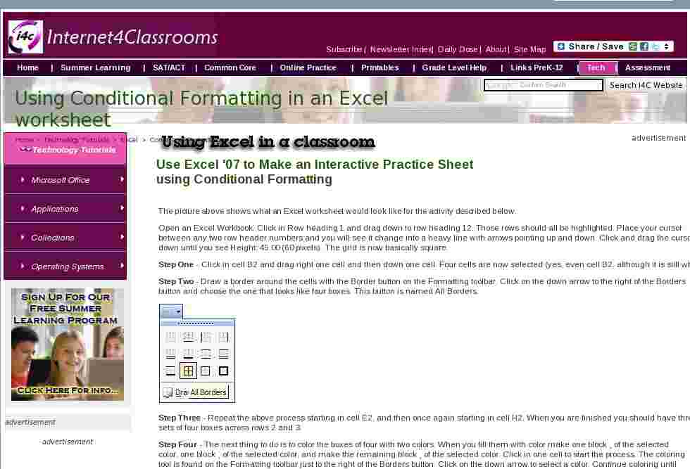
The picture above shows what an Excel worksheet would look like for the activity described below.

Open an Excel Workbook. Click in Row heading 1 and drag down to row heading 12. Those rows should all be highlighted. Place your cursor between any two row header numbers and you will see it change into a heavy line with arrows pointing up and down. Click and drag the cursor down until you see Height: 45.00 (60 pixels) . The grid is now basically square.

Step One - Click in cell B2 and drag right one cell and then down one cell. Four cells are now selected (yes, even cell B2, although it is still white).

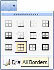
Step Two - Draw a border around the cells with the Border button on the Formatting toolbar. Click on the down arrow to the right of the Borders button and choose the one that looks like four boxes. This button is named All Borders.

Step Three - Repeat the above process starting in cell E2, and then once again starting in cell H2. When you are finished you should have three sets of four boxes across rows 2 and 3.

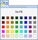
Step Four - The next thing to do is to color the boxes of four with two colors. When you fill them with color make one block ¼ of the selected color, one block ½ of the selected color, and make the remaining block ¾ of the selected color. Click in one cell to start the process. The coloring tool is found on the Formatting toolbar just to the right of the Borders button. Click on the down arrow to select a color. Continue coloring until the three boxes are colored ¼, ½, and ¾ of the color you are using. Next, select a second color and fill the remaining fractions of the three blocks with the second color.

Step Five - Click in the left cell immediately below the first box and type the letter A. At the cell below left corner of block 2 type the letter B, and then type the letter C below block three.

Step Six - Click on the letter A, then hold down the Ctrl key as you click on each of the other letters. Change the font size to 36. This can be done with the pull down arrow on the font size block.

Step Seven - Click in cell B5 and type the words, Which is ½ blue? (or your chosen color). In cell B6 type Which is ¼ blue? (or your chosen color), and in cell B7 type Which is ¼ yellow? (or your second chosen color).

Step Eight - Click in cell B5 and drag down to cell B7 to select all three cells. Use the font size block on the Formatting toolbar to change them to size 20.

Step Nine - Click in cell G5 and drag to cell G7. Use the All Borders button to draw boxes around all three cells. Then, use the Fill Color bucket to fill all three cells with light yellow.

Step Ten - Click into cell C8 and type, “Type answers in the blocks, correct answers will turn green.

Step Eleven - Click and drag to highlight all three of the light yellow boxes. Use the Font Size box to change font size to 20. Step Twelve- Save your work before going further.

Setting conditional formatting in the Answer boxes

Step One - Click into cell G5 (the first light yellow block). Decide if the answer is A, B, or C before going further.

Step Two - Select the Format menu from the top, slide down to Conditional Formatting and click one time.

Step Three - In the Conditional Formatting window use the pull down arrow to make box 2 read equal to and then in the block to the right of that type the letter B (if that is the correct answer on your worksheet). On the right side, click on the button that is labeled Format, and then in the Color block use the pull down to select Bright Green. Click OK to come back to the Formatting window, but do not click on the Conditional Formatting window yet. Next choose Add (the leftmost button on the last row) and this time make the cell contents not equal to . Enter B just as you did before. Next Click on the Format button and change the color to red.

Step Four - Move to cell G6 and continue the same process until conditional formatting has been set for cells G6 and G7.

Step Five - As a last step, let’s remove the grid lines from this worksheet. To remove the grid lines, go to the Tools menu, slide down to Options and click one time. On the View tab, in the bottom left corner there is a checkmark by the word Gridlines. Click in the box to remove the check mark and then click OK to return to a blank worksheet.

Step Six - Save your work.

Sample worksheet on this topic