Using Excel '07 to Make a Venn Diagram

Excel 2007 has a large number of graphic organizers built in. On the Insert tab in the Illustrations area, click on Smart Art to see the large number of graphic organizers possible with the new Office 2007. One of the thirty-one available organizers in the Relationship subdivision of Smart Art is a Venn diagram. This module will not use the pre-designed Venn, we will use Shapes to create our own.


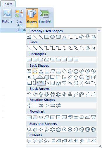
Step One - Open Excel. When the worksheet opens, remove the gridlines. This can be done by using the Page Layout tab or the View tab. On the Page Layou t tab in the Sheet Options section there is a checkmark in the box named View under Gridlines . On the View tab in the Show/Hide section there is a checkmark in the box named Gridlines . Click on the checkmark to deselect that option and you will remove gridlines from the worksheet.

Step Two [draw a shape] - Select the Insert tab by clicking on the word Insert below the Quick Access toolbar. Click on Shapes in the Illustrations section to see all available shapes. We will use the Oval shape which is the second shape on the first row of the Basic Shapes list. Click on the oval and release the mouse button. This is not a click and drag operation. Move the cursor onto the blank worksheet. The cursor changes to a slender plus sign or cross hair shape. This is the drawing cursor. Click and drag diagonally to draw a circle that fills the left half of the worksheet. To make a perfect circle, hold down the Shift key with one hand while you drag the drawing cursor. Release the mouse button before you release the Shift key or the shape will be an oval rather than a circle.

[ this image has been simplified ]

Step Three [duplicate the shape] - Rather than drawing another circle we will make an exact duplicate of the one that was just drawn. If the circle is not selected (a thin blue line makes a box around the chape when it is selected) click one time on the circle to select it. Hold down the Ctrl key and press the D key one time to duplicate the shape. That is the same as copy and paste, but it involves only one step rather than two.

Step Four [move the shape] - Click and drag the new circle to the right until the circles overlap in the classic Venn format. The circles overlap, but you can not see the overlap because both circles are full of color.

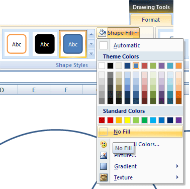
Step Five [format the shape] - To make our Venn diagram ready to use we must remove the color from both circles. Hold down the Shift key and click on the circle that is not selected. This allows you to select both of the circles and format them at the same time. When you drew the first circle, the Excel ribbon changed to display a new tab; the Format tab under the Drawing Tools . If you have clicked away from the circles you will move back to the last tab selected. However, the Drawing Tools will still be only a click away. With both circles selected, click on the Shape Fill button in the Shape Styles area select No Fill .

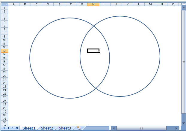
Step Six [use the Venn diagram] - The black rectangle below is a cell on the worksheet; cell H13. To select any cell to begin typing, click into the cell and type.

Note: Office 2007 does have a Venn Diagram ready to use. Select the Insert tab, look in the Illustrations section and click on Smart Art . Scroll down to the Relationship list and select Basic Venn , a three circle Venn diagram. I removed one of the circles to make a Venn similar to the one we drew.

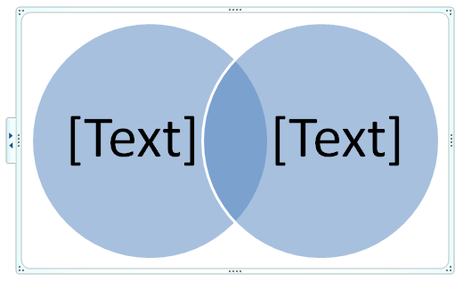
This Venn diagram is not as flexible as the one we drew and seems to be more for displaying large ideas rather than brainstorming comparisons of two things;

Let us know if you have any other ideas for using this feature of Excel.